Quantum News Channel 1

Last time, we talked a little bit about entropy and classical information theory. If you haven’t already, check that article here. It gives a good introduction to this one, introduction so good that I have serious trouble writing another one here. Hopefully this short introduction will be over soon.

At the end of the previous post I mentioned that classically, probabilities are quite simple and that it gets much more complicated in a quantum case. Why exactly? And what is the “quantum case”?

Quantum mechanics is the language of modern physics. It is a base on which more complicated theories can be built, for example regarding behaviour of particles and fields, describing new phases of matter, interactions of lasers and atoms, or collective motion of solid materials. But all these theories rely on quantum mechanics. Some people, like Scott Aaronson [1], claim that quantum mechanics is at its core a theory about probability and information. It is just a more… complex one. Literally. As he puts it in his book:

“But if quantum mechanics isn’t physics in the usual sense – if it’s not about matter, or energy, or waves, or particles – then what is it about? From my perspective, it’s about information and probabilities and observables, and how they relate to each other.”

Let’s say you have a box, and in that box you have, say, 3 oranges, 5 apples and a pear. You reach inside and you grab one fruit. It is easy to see, because we are used to classic probability theory, that a chance of grabbing an orange is , a chance of getting an apple is , and a pear . We just divide the number of fruit of the requested kind by the total number of all fruit in the box. One particular property of this is that these probabilities sum to . What does that mean? Well, a sum of probabilities of getting an orange, an apple and a pear is a probability that you will get either an orange, an apple or a pear when you reach in and grab a fruit. Provided our assumptions – that you will indeed grab something and there are no other fruit in the box, this will obviously happen. It is called a sure event. This a fairly obvious, but crucial property – the sum of probabilities of all disjoint events, all different possible things that can happen, I mean, really all of them, must be equal to 1, because “something” will always happen.

Scientists started developing quantum mechanics because they encountered a range of peculiar phenomena which their classical theories failed to account for. Now we know that the fundamental reason behind this was that the classical probability theory fails to describe things happening at very small scales. Classically, if a probability of one event is and a probability of a different, disjoint event (think about grabbing an orange vs grabbing an apple) is , the probability that either one of these independent events will happen is the sum of the probability of each one happening on it’s own i.e . This in general doesn’t work in quantum mechanics.

In the quantum world, probabilities are changed to something called probability amplitudes. We can add probability amplitudes of two similar events to get an amplitude of a joint event (either the first or the second thing happens). Amplitudes are different from probabilities – first, they can be negative! What is more, it can actually be shown that for this theory to be consistent, amplitudes will sometimes have to be complex numbers. Second, it’s their squared moduli (if you are not familiar with complex numbers, think about squared modulus as a “square” of a complex number which ends up being a real number) what adds to , not the amplitudes themselves. In other words, if we know that one set of amplitudes describes everything that can happen, a sum of squared moduli of these amplitudes will be exactly , again, because “something” will always happen.

What exactly we are supposed to be adding? Should it be the squared moduli or the amplitudes themselves?

Any quantum system can be described as being in some state. That state is a mixture of several basis states, as described above. We are allowed to play with that state. Change it, make it evolve. We say we apply quantum operations, make the state interact with the enviroment, apply magnetic fields, shine light onto it. The state then changes. In particular, these operations might involve two different states at least partially evolving into the same state, with different amplitudes. Or the same state evoling into some other state in two different ways! In that case, to find out what is the total amplitude of that state in the mixture, we add the amplitudes coming from different processes, but ending up in the same state. Then the resulting amplitude is the amplitude of that state.

After these operations, we usually want to measure the state. By measuring, we ask a quantum system the question: which state are you in? But this question is not an open one! It is a close one. We have to pick all the possible answers we can get. The number of these answers is limited to the dimension of the system. For a single qubit, the dimension is two, so we can only get two different answers, the system can only tell is that it is in one of the two states that we pick. But if the state is somewhere in between, we are forcing it to change by performing the measurement, we are forcing it to become a different state, one of the ones we picked. The probability of that happening is the square of the amplitude associated with that state. If we then prepare another, identical state, and perform the measurement again, we might get a different answer, even if we do everything exactly in the same way. This is because quantum mechanics is instrinsically probabilistic (well, according to most interpretations at least). If we want to then calculate the probability of getting either one or the other states, we enter the classical zone and we first square the amplitudes of each state and then add these squares for the joint probability.

For example, let’s imagine a quantum particle that travels from a point A to one of the points B or C. These are somehow the only two points where it can end up. On its way, it can either travel through point X or point Y, but that is not known – we never learn which path was taken by the particle, but we do know where it ended up in. We thus add amplitudes of particle travelling through X to B and through Y to B too get an amplitude of ending up at point B. And then we do the same for point C, add amplitudes of travelling through X to C and through Y to C, and then we square the whole thing to get the probability. Now, if we add the two squares, this will add up to one. This is because in macroscopic scale probabilities are classical, and because B and C are different states,  easily distinguishable, the classical rules apply.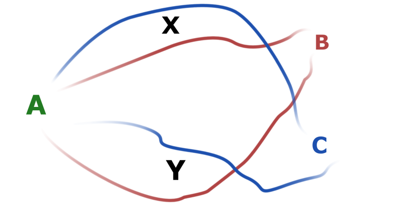

Because these amplitudes are in general complex numbers, it is possible that the amplitude of getting through X to B and an amplitude of getting through Y to B are opposite numbers and they add up to 0! In which case the existence of two different paths leads to a complete cancellation of any possibility of a particle ending up at B. This is the paradox scientists were struggling with: if you only have one path, the particle can end up at B, if you have only another one, the particle can still end up at B, but when both paths are available, it becomes impossible suddenly.

This is resolved by using an alternative probability theory. In fact, this assumption about probabilities, that they can involve negative numbers is the only one you need to make to recreate quantum mechanics. The fact that probabilities work differently than we previously thought is what underlies most of the modern physical theories.

But okay, we wanted to talk about information, right?

To talk about quantum information, we need a fundamental portion of it. In classical world, it was called a bit, a number, either 0 or 1. Something that either is or isn’t. It was realised by a physical system, which could remain in two separate states, for example magnetized or demagnetized, black or white, up or down. It is important to remember information is and always was physical, needed a physical realization. In the quantum world, we have qubits. Qubits
also are physical objects, that can occupy two independent quantum states, which are traditionally denoted as  and . These strange asymmetric brackets are ‘kets’ from Dirac bra-ket notation, it is just a way physicist write quantum states. But qubits, as quantum objects, can also occupy other states, which are linear compositions of the two states above, or the states “between” them. In other words, it might be in a state   , where and are numbers. Complex numbers, in general. These are exactly the amplitudes I mentioned earlier. A system in this state is called a superposition, exactly because it is a sum of two different states with some amplitudes. Superposition is a kind of subjective concept – a quantum state is represented as a vector in some space, but whether this vector is a basis vector or not depends on the choice of basis, for example, mentioned  and states are called computational basis, but there are many other bases that can be used depending on circumstances. Therefore the same state might be regarded as a superposition or not depending on from which angle we are viewing the system. The important bit is, once you settle for a basis, for a particular angle from which you want to view your quantum system, the superposition states are possible. The basis states, whatever you choose them to be, are not going to be the only states your system might reside in.

 

 

 

A quantum system may remain in such state as long as it is not disrupted in any way. The problem is, we don’t usually know what the state is exactly. And trying to find out – a measurement, is already a disruption of some sort, because it has to involve some physical process that interacts with the state, and such states are really fragile. When we see things, photons need to reflect off them and reach our eyes, when we hear them, air particles vibrate on the way from the source to our ears, when we touch things, electrical signals travel through our body to our brains. The interaction has to be there for anything to be observed, and really what is important is that it happens, not that its products reach our bodies. In other words, the existence of a human or other conscious being is not needed for a measurement to be conducted. Unfortunately, it is a common misconception among laymen and that needs to be stressed.

One of the reasons quantum information is so different from classical is a mysterious quantity that has no equivalent in a classical world, entanglement. Entanglement is a property of a system consisting of many particles, and it is a peculiar way the states of particles this system consists of are correlated. An example of an entangled system is a pair of photons of opposite polarisations. Before measurement, we know that the polarisations are opposite, but we don’t know exactly what are their directions. After we measure only one of these polarisations – we can measure it in whatever way we want, along any axis we choose, and that way will affect the result, the second one becomes defined and exactly opposite to the first one! It turns out that entanglement has many peculiar properties, some of which are not yet completely understood.

Classically, systems that are correlated, can be correlated to different levels, some pairs of variables are correlated very strongly, and some only a little bit. For example, there is a very strong correlation between your age in years and your age in minutes – it is basically the same quantity, but in different units. But there also is correlation between the age and height across children – older kids are going to in general be taller, but people have different heights, because that is partially determined by genetics, so younger children might be taller than older ones if their parents are especially tall. So there are different levels or degrees of correlation even classically. Similarly, we can find that there are different degrees of entanglement. Some pairs of systems can be strongly entangled, and some only to some level. A fascinating result is that it can be extracted from physical systems which are not completely entangled to form a fewer number of systems which are, so it can be treated as a resource. What’s more, entanglement of a single particle is limited – if the particle is completely entangled with another particle, it cannot be entangled with anything else. [3] It is called monogamy of entanglement and we can see that it is completely different from the classical correlation, because classically, you can have as many systems strongly correlated with each other as you manage to create. This is because entanglement is not just statistical correlation. It is much stronger, because in quantum mechanics you can measure the state of the system in many different ways, and entanglement forces correlation in each of these measurements, not just one.

That is why quantum systems can be correlated much more than classical systems because of entanglement. This is how physicists have confirmed that the world cannot be purely classical, that is, levels of correlation which are classically proven to be impossible are actually possible in practical experiments involving highly entangled particles!

For example, think about a following game. There are two players, Alice and Bob, who collaborate to win. Each of them has a standard deck of cards and every turn, draws one card from the deck and doesn’t show it to the other player. Then, basing on the card that they’ve drawn, each of them decides either to push a button or not. They have to make their decisions simultaneously, so that they are not affected by the other’s decision. Now, if they both pushed their buttons or they both haven’t, they win provided at least one of the cards they’ve drawn was red. But if one of them pushed their button and the other have not, they win only if both their cards were black.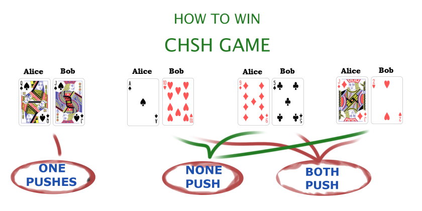

It is quite easily seen that they can win in  of games if they just never push their buttons ever, because there is a 75% chance that at least one of their cards is going to be red. It can also be shown that it is the highest overall probability of winning for any strategy they are allowed to come up with.

However, if the choice of a card from the deck is determined not by sheer luck, but by a clever quantum measurement of a half of entangled quantum state Alice and Bob share between each other, the probability can go up to about 85%! That beats the classical result which can be proved to be correct. Both Alice and Bob only measure their own qubit, which has exactly 50% chance to be in one of two states, what can be associated with a card being either red or black, so the probabilities work out. Also, they can be very far away from each other, so that for any information from the other party was to influence their decision, it would have to travel much faster than the speed of light in a vacuum. However, despite all this, the quantum nature of entanglement still bumps up probabilities to 85%! That has been confirmed experimentally, and it is a realization of one of the Bell inequalities. These inequalities are rigorous statements, which reality would have to satisfy if it was purely classical or at least local, what means, there would be some local hidden influences, which cannot be seen directly, but which change the way it behaves. Experimentally, however, it was in most cases confirmed that it doesn’t satisfy those, and actually it comes close to what non-local quantum theory predicts.

Entanglement is just one of the resources that quantum information theory utilizes, and which make it much richer than classical theory. What the quantum information theory tries to do is to find out about what other types of information are there in the quantum world, because there are certainly more than in the classical world, what other types of information processing are there, and then what can we actually do with those and what exactly are the limits we have to obey while performing those processes, how do this different types of information change, are created and then destroyed.

The researchers managed to find many, many more such types, listing them all here would not be possible, so for now try to think about this and come back in two weeks for more!

In the meantime, you can read more about entanglement and quantum mechanics here:

1. An excellent semi-popular book by Scott Aaronson about information and computation “Quantum computing since Democritus” with more details about the approach that I have basically stolen from him.
2. Bennett, Charles H.; Bernstein, Herbert J.; Popescu, Sandu; Schumacher, Benjamin (1996). “Concentrating Partial Entanglement by Local Operations”. Phys. Rev. A. 53: 2046–2052 – the first paper about entanglement distillation.
3. V. Coffman, J. Kundu and W. K. Wootters, Phys. Rev. A 61, 052306 (2000), a paper that introduced monogamy of entanglement.
4. The “Bible of quantum computing” with chapters about quantum mechanics and entanglement “Quantum computation and quantum information” by Michael Nielsen and Isaac Chuang
5. Definetely also check out Scott’s blog: https://www.scottaaronson.com/blog/
6. Very short description of quantum computing, from one of research group at University of Strathclyde, I am including it because it is short and I took one of the images from this site, I hope they don’t mind because it was really nice.

 

The physics of information and uncertainty

They say we live in an information age. That usually refers to the fact that communication between humans residing across the globe is much quicker than it used to be and that value is more than ever associated with knowledge. But what is information actually?

Information is… just a word. An abstract concept! The real question we should be asking here is about things that can be seen or measured. Instead of thinking about what “information” means, we should be thinking about what does it mean to “inform” someone of something, we should focus on a verb, because it has a definite, physical meaning.

So that when you inform someone of something, you send them some pieces of knowledge, change their perception of reality, add some new element. With useful information you can often change your mind about what you think about chances of certain events occurring. With more data, we make our guesses about reality more effective.

Perhaps you need to find a person called Jamie in a crowded room. You don’t know anything about that person, it can be anyone. Maybe someone tells you that Jamie is a man, not a woman, which limits your choice to about half the people in a typical room. Then you might be told Jamie is over 40 years old, which then filters out younger men and boys present, if there are any. Finally you may learn Jamie has a moustache and wears a red t-shirt, which limits your choice to just one person, who you then approach.

Each of these messages contained some information, because it let you change your perception about who is that person you are looking for. A bit more formally, it let you update the probability of finding Jamie by asking a random person if they are him. Or in yet other words, it limited your uncertainty about the stranger’s identity to some degree.

However information might seem a volatile, abstract concept, every transfer of information involves a physical process. You might hear it, which means that particles of air vibrate in a specific fashion that reaches your ear, or see it, when photons enter your eyes and then signals travel to your brain which interprets it, or get it in some other way. Storage of information also requires physics, a message might be written down on a piece of paper, or as a sequence of magnetized and demagnetized segments on a disc, but it has to be physically contained somewhere to exist. We say that information is physical.

You might still think, though, that information is then just a concept humans adopted for themselves, that for physics there is no difference between a sheet of paper with words in English written in black ink and a similar sheet of paper with similar amount of ink on it. And it would be kind of correct, but only kind of.

Two configurations like the ones above can be equivalent in a sense that they are equally probable, if you sprinkled some ink over the paper there is an equal chance that it would form these exact shapes. However, the catch is in the word “exactly”. Surely, sheets with random dots on them constitute a much wider category than sheets of paper with words on them. Therefore the chance that randomly sprinkled ink would form a word – any word for that matter – on a piece of paper is much lower than that it would form something that doesn’t look like a word. So even though a probability of getting one exact configuration is the same as a probability of another exact configuration, thinking about these exact configurations – microstates, as they are called in statistical mechanics – is not want we want to do here. Words appear less random than dots simply because there are much fewer configurations that resemble words! In the same way, if we tossed a coin 6 times, and got a following sequence: H,H,H,H,H,H, it would look to us much less random than a sequence like H,H,T,H,T,H for example.

So far, this might seem like juggling words around. To get more physical, think about gas in a box. Say there are about particles in that box, and so there is a plethora of exact configurations of their positions and momenta, the parameters that are in principle needed to fully, exactly describe the system. In most of them, the particles would appear to be almost evenly spread across the box. Now, let us think about the unusual configurations, when all the particles are in the right half of the box, and are randomly spread there. There are much fewer such configurations, so that is much less probable. How exactly?

If we assume the box is divided into equally probable little spaces the particles can occupy, no matter how big these spaces actually are, then there are configurations in the case when particles can be spread out across the whole box. But in a half of the box there are only spaces, what means only configurations – a square root.

Physicists like to talk about something called an entropy of each category. Because it should not matter how small these spaces actually are, the change in the numerical description corresponding to a change between a container filled with gas particles and the one half filled should be the same, the earliest equation for entropy, written down by Boltzmann, involves a logarithm, which deals with that issue:

Where is entropy, is a number of possible states – arrangements in this case, in general this also involves momenta, and is a Boltzmann constant. This equation shows that the entropy of a half filled container is a half of the entropy of a full container. It however assumes that each microstate has an exact same probability to occur. If the probabilities are different, equal to , the entropy changes to Gibbs’ form, given by

This is a bit different, before we had number of states, a large number, now we have probabilities, which are small. However, we notice that Gibbs’ formula becomes Boltzmann’s formula if we replace all -s by , one over the number of microstates, which is a probability of a single microstate if they are all the same. This is because the minus sign in front inverts the argument of the logarithm.

Entropy is a key concept here. The second law of thermodynamics, known since XIX century, states that in any isolated thermodynamic process, the total entropy of the system can either stay the same or increase. It can never decrease, although entropy of certain parts of the system might, on the expense of greater increase in other parts. If the system evolves via spontaneous processes, each increasing its entropy, it will finally reach the maximum allowed entropy state. In other words, if we place gas in half of the container and release it, it will fill the whole box. We can break an egg, but it is impossible to put it back together. Order is in general harder to achieve than chaos. Entropy is a measure of how much uncertain we are about the system. If we know everything – the entropy should be zero, if we know nothing at all, it should be maximal. Therefore entropy is a measure of information, the more information you have, the smaller uncertainty and the smaller entropy.

Thermodynamics connects entropy to work and heat, and this is how physics distinguishes information from the lack of it. Essentially, if you want to achieve greater order in your system, smaller uncertainty, you need to expend some energy for that purpose, do some work, which will then turn into a form of energy that cannot be collected back in its entirety. To create new information, you need to spend energy, which might not be totally regained after that information is destroyed. Also, information tends to wear out over time, when spontaneous processes increase entropy, gas travels and fills the box by itself, random errors erase bits in a computer storage, quantum system lose coherence due to interaction with the environment – we’ll get to that!, we lose some knowledge about the system that we previously had.

Okay, we’ve got entropy. Entropy changes the game a little bit, we now know that physics cares about information in a sense. Now, let’s move on to answer a question about what information is in more detail.

In the middle of the XXth century, American mathematician Claude Shannon was thinking about communication. He defined communication as an act of transfer of messages, exactly or approximately, from one point to another. He was interested in, generally speaking, the efficiency of such transfer. He was considering something called communication channel, at one end of which there is an information source and on another, there is a receiver. The source generates symbols from some alphabet, arranged in words. The source can be imagined as a human writing down a message for example. Then, the message is encoded into another language, the language of the channel. It might be a series of ones and zeroes, or dots, lines and spaces of a telegraph, or specific sounds, or even clouds of smoke. The point is, we don’t transfer our messages directly over the large distances, we need to encode them first. The person receiving the message has to then decode it to understand it. Usually, the transfer is costly, there is a cost associated with a transfer of each symbol through the channel. Therefore when we encode, we want to be as concise as possible, but still retain the whole message we want to communicate.

The goal of Shannon was to show what are the limits of efficiency of such coding and decoding, to find out how many words can we squeeze through a channel to still be perfectly understood on the other end. The reason we can do this at all is because languages are somehow redundant, letters we use come up in certain patterns called words, and in those patterns only. Words form some grammar, which has to be obeyed for the whole sentence to make sense. A random sequence of letters is very unlikely to mean something for a human. Making use of the correlations might decrease lengths of encoded messages. For example, if you receive letters e,x,p,e,r,i,e,n,c in that order, you are almost sure that the next letter will be e. So when e comes, it doesn’t carry any new information – it might be dropped without influencing the understanding. Also, some letters or words are used more often than others, what means that encoding them with shortest codes will minimize the length of the encoded message. In old telegraph codes, a letter e, the most frequent letter in English texts, was encoded with a single dot, the shortest possible signal that could be sent.  Basically, there is a room for improvement. Shannon’s idea was to find out an objective measure of an amount of information carried by typical messages in a given language, and compare that to the maximum amount of information that can be transferred through the channel, and therefore find out the maximum rate of compression that allows to transfer the message most efficiently.

And what is this measure of information? It is entropy! It is not exactly the same entropy as in thermodynamics, however it is inspired by it and it behaves similarly mathematically. Let’s first paint the initial picture. In the first approximation, we consider a source to generate the letters randomly, following certain probability distribution. That means we are skipping a part of its structure for now, we neglect for example the fact that certain letters follow others more often. We only focus on how often each letter appears in text on average. Of course, the source doesn’t actually generate random letters, as in a popular meaning of a word “random”. However, the frequencies with which letters appear in the text are defined and reflect the given probabilities. That is all we need for now.

If letter number appears with probability , then entropy of a source is:

The same equation as for Gibbs entropy! What this entropy function reflects is a minimal average number of bits needed to encode one letter of a message generated by a source. In other words, if our message is letters long, with the most efficient coding we are going to need on average bits to encode it.

A simple example might be as follows, imagine a source, a language, in which there are only three letters, A, B and C, and A appears twice as often as B, which appears as often as C. That means , . We can calculate the entropy of this source:

That means we need at least $\frac32$ bits per letter to encode a message here. How can we do that? First, we keep in mind that we should try using shorter codes to represent more frequent letters. So code for A should be the shortest. Why not just use one bit to represent it, then? We can set 0 to represent A, then a string 10 to represent B and a string 11 to represent C. Decoding such message will then look as follows. We consider the first bit, if it’s 0, we write A and move on. If it’s 1, we check the next one, if it’s 0, we write B and if it’s 1 we write C and then move on.

How efficient is this? We can see that because A basically takes 50% of the message, and letters B and C take 25% each, an average of bits will be 50% + 25% . Exactly equal to the entropy value! Basically, the number of bits we aim to use for each letter should be as close as possible to , where is the probability of that letter. Then, when we calculate the bitrate, we recreate the entropy function.

Entropy was then again used as a measure of information, however in a slightly different way. We once more had probabilities, reflecting our lack of knowledge about what will come next, this time however the higher entropy of a message, the more information was there in the message. So there are two ways to think about it, either entropy is an average information learnt from a letter, or an average uncertainty about what the letter will be before we know it – which is actually the same thing, but at a different point of time.  A message which is constructed from an alphabet containing only one letter, no spaces, no nothing, doesn’t actually carry any information, and has entropy of 0. But we also don’t need to spend resources to transfer that message anywhere, we already know what it is.

We wanted to reduce redundancy to be more efficient, but sometimes we actually would like to introduce some. For example, if a communication channel we are using is somehow noisy, there can be errors introduced in transfer, and we want to make sure that regardless of these errors we can actually be understood. If during transfer some letters have small chance to change to other letters, you might receive, for example, a word ‘exparience’. There is no such word in English, but you guess it was supposed to be ‘experience’. The redundancy is good, because it lets us recover a distorted message. There are different types of noise and some of them are worse than others, so different levels of redundancy will be needed in each situation. The question is, how much redundancy is enough?

Let us focus on a specific case, of which generalizations we will not bother here, when an encoded message consists of 0-s and 1-s, and a probability that 0 changes randomly to 1, or 1 to 0 is equal to some . Then, 0 staying 0 or 1 staying 1 has a probability . It can be then shown that if we introduce so-called binary entropy function the rate of compression has to be proportional to . The closer is to 1, the more bits we need in order to transfer the message. This makes sense, corresponds to , and that means we can have no idea whatsoever about what the message actually was, as exactly a half of the bits are flipped, so the message looks like a completely random string.

So here entropy is once again a measure of uncertainty, lack of knowledge about the system.

Information has a lot to do with probabilities, chances of certain things happening. The closer are probabilities to 1, the more certain we are, so the more information we have. Even though obviously information theory was developed to enormous degrees, this connection is quite simple, because classically, probability is simple. It is just a number between 0 and 1, which can be interpreted either as a fraction of events that satisfy some special criteria, or our degree of certainty that a single event is going to satisfy them, but mathematically, it is a number between 0 and 1.

This will get tremendously more complicated when we introduce quantum mechanics. But worry not! I will be your guide… in my next essay here.

For now, you can get ahead of me and check out some useful reading:

1. Any thermodynamics textbook to learn about entropy in physics – good one is “Concepts in thermal physics” by Stephen and Katherine Blundell
2. The “Bible of quantum computing” with an introduction about classical information theory “Quantum computation and quantum information” by Michael Nielsen and Isaac Chuang
3. An excellent semi-popular book by Scott Aaronson about information and computation “Quantum computing since Democritus”
4. Definetely also check out Scott’s blog: https://www.scottaaronson.com/blog/
5. A more philosophical treatment in a book “Quantum Information Theory and Foundations of Quantum Mechanics” by Christopher Timpson

On Mathematics, Physics and Truth

What is the role of truth, and by extension philosophy, in physics and in mathematics?

This question was carefully examined at the turn of the 20^th century when, faced with a plethora of strange and counter-intuitive results, it was deemed necessary to come to terms with the role of truth in each field. What is the influence of mathematical results on our picture of reality? Is nature really whatever our physical models say it is? What makes a theory “acceptable” in mathematics or in physics?

On the mathematical front-lines, David Hilbert, following Riemann, Helmholtz, Clifford and Poincaré, championed a view which challenged the concept of truth insofar as mathematics is concerned. He argued that the metaphysical truth of a statement is irrelevant to mathematics, which instead ought to be concerned purely with the logical consequences of that statement.

To clarify what I mean by “metaphysical truth,” let us consider an example: in his famous works on Geometry, Euclid begins with the statement that “a point is that which has no part”.  Is this true? Does a point exist? We may take two different roads to answer this question.

On the first road, we believe that in physical reality there exists such an entity which we are attempting to describe with our definition. In this case, we must somehow show that this entity exists and that our definition captures it adequately.

On the second (modern) road, we assert that, in some hypothetical reality, there exists an entity called a point which is precisely described by our definition. In this case, the point exists in our hypothetical reality by assertion. Whether this hypothetical reality coincides with physical reality is out of the question – a matter for a physicist or philosopher to decide upon.

Each assertion we make within our hypothetical reality is more or less an assumption on which we will build all of our deductions. It’s natural to wonder if we have made a redundant assumption, in which case we simply need to prove that our redundant assumption is actually just a consequence of the others.

In any such hypothetical reality, we will find that the truth of any mathematical statement therein is tantamount to the truth of a set of irreducible statements, the things we must assume which are formally known as axioms. This set of axioms is essentially the backbone of any mathematical construction within that reality.

Within Hilbert’s paradigm, mathematics evolved into a study of consequences which dismissed the notion of metaphysical truth. Any set of axioms is deemed permissible with one caveat – the axioms must be consistent¹. In other words, if we can prove the truth of two contradictory statements with our axioms, then they cannot all be simultaneously true. Such a construction is not allowed since it is demonstrably self-contradictory and therefore logically inconsistent i.e. mathematical heresy.

A famous example is given by Russel’s paradox: imagine there is a big list of lists that don’t list themselves. Does the big list contain itself?

If it does then it must be a list that lists itself so it cannot be on the big list.

If it doesn’t then it is a list which doesn’t list itself meaning it should be on the big list.

Wait a second. Being on the big list means it isn’t on the big list and not being on the big list means it is on the big list: PARADOX.

Clearly, such a construction cannot exist and mathematicians took great care to adjust the axioms of the reality of mathematical lists (set theory) to prevent such constructions from existing.

An important question to ask at this point is, can an axiom be true in one consistent reality but false in another? Well, it turns out that some mathematical constructions may require it to be true, others may require it to be false, and some may even be independent of it altogether (consistent whether it is true or false).

The classical example of this (and indeed the reason why this matter was debated in the first place) is the fact that Euclid’s parallel postulate is not a necessary axiom for consistent geometries. The postulate asserts that, given a straight line and a point not on this line, there is exactly one parallel line which goes through this point. Seems absolutely true, doesn’t it?

In a stroke of genius, Poincaré showed that Non-Euclidean geometries (where the parallel postulate fails) are as consistent as Euclidean geometry by constructing a dictionary allowing one to translate the results of one geometry into the results of the other and vice versa. As a result, if people accept that Euclidean geometries are legitimate then they would have to accept that Non-Euclidean geometries are equally legitimate.

In summary, we see that an axiom is more or less a definition, a rule of a mathematical game: asking if the rules of the game are true is like asking if the rules of Monopoly are true. The mathematician’s job is purely to determine how the game unfolds, and not to concern themselves with the rules of the game, no matter how weird or whacky. Provided that a move cannot be both correct and incorrect according to the rules (imagine the arguments) then it is acceptable as a game. This is the “shut up and prove” ethos.

However, if we wish to apply mathematical results to solve some problem, the approach becomes radically different.  We must first model the problem by making several idealisations and assumptions. We then attempt to understand its internal structure, that is the variables of the problem and the relations between them, determine if it has a well-defined answer or if we require additional assumptions to arrive at a unique answer and so on.

We may find that the problem can be modelled within several mathematical systems allowing us the freedom to choose the most convenient or simple one to arrive at a solution. For example, we may be asked to prove some relation which may be a horrible task when performed analytically while being astonishingly simple within a geometric framework. Perspective is key.

As a result, physicists are not so free to evoke any set of mathematical axioms to describe natural phenomena. The truth of axioms is a real concern to physicists since their veracity is ultimately decided, directly or indirectly, by experiment.

An important point to make here is our models are mainly meant to supply us with useful information requiring as little ink as possible. If we are attempting to model a stone dropped two metres in the air, it makes sense to assume that there is no air resistance since it has such a small effect. However, if it were falling 100m, then our models’ predictions would quickly depart from reality.

We would have to add some fine print to our model saying e.g. “this prediction is valid within a length scale of up to 20m.” Interestingly, one can go so far as to say that it is a law of physics that stones will fall according to this model in a range of up to 20m, however that would be a waste of a law for one important reason: it follows from other laws which hold over a much larger scale of lengths and speeds.

Does this mean that those laws are not “really” true? Such a question is on par with the question posed of mathematicians with regards to constructions with a slight difference. In the realm of physics we have to decide if “really” true means that this model is exactly what nature is or if “really” true means that nature behaves in a manner consistent with this model, where applicable.

As a rule, experiments do not tell us if a model is correct, quite the opposite: they tell us if a model cannot be correct. We cannot know if an electron is truly a spherical entity or some incredibly complex entity that behaves in a manner entirely consistent with spherical entities (as in there is no experiment that we can conceive of or perform that allows us to distinguish between the two). We can, however, know that an electron is not something which behaves in a manner that is inconsistent with spherical entities.

When we say we know what an electron is, we, in fact, mean to say that we have discovered an entity which has certain properties, and by properties we mean relations; expressions of how this entity interacts with other entities. We call this entity the electron. Our model of the electron is a representation of the knowledge we have thus far acquired with regards to its behaviour, and we have no means of determining if this knowledge is complete.

Should physics then be concerned with the true nature of the substance it describes, or should it be content with modelling the behaviour of said substance and not ask if the model itself is metaphysically true?

To answer this rather dramatically, suppose that someone claims that gravity is really a manifestation of mass spirits. They then make claims about the behaviour of mass spirits which makes them entirely consistent with Newtonian gravity as far as predictions are concerned. Suppose further that one of their statements about the theory of mass spirits is a definition that “the spirit is a projection of the living soul of matter”.

As far as a physicist is concerned, this statement is meaningless because it is not testable. It is an irrelevant and vague complication the neither helps nor harms the act of prediction. One could just as easily make any number of such claims which are consistent with the theory of gravity but differ on such arbitrary untestable statements.

We have decided that experiment is the ultimate judge of physical truth. Experiment sheds no light on the nature of the things we study, it sheds light only on the relations between the things we study. It cannot distinguish between theories which agree on all predictions. Such theories are equal in the eyes of physics insofar as their predictions, and ultimately the relations they describe, are all the same. Any other details are completely irrelevant since there is no means of testing their truth or falsehood. As such, they are regarded as being useless embellishments and are therefore discarded.

As Poincaré puts it,

“The aim of science is not things themselves, as the dogmatists in their simplicity imagine, but the relations between things; outside those relations there is no reality knowable.”

Physicists had to face yet another difficulty in this period. It was previously assumed that it is possible, at least in principle, to measure any observable quantity to arbitrary precision – the only limitation being how well the designed the experiment or how skilful the experimenter.

For example, there are fundamental limitations to how precisely one can simultaneously measure certain observable quantities. In other words, we may know precisely that the electron is located at this point, but the price of this knowledge is a total lack of knowledge as to what its momentum is and vice versa.

Now comes a key question: does the electron actually have a specific momentum and position simultaneously even though there are no known experiments allowing us to observe them?

Should physics be concerned with whatever lies behind the scenes of observable reality, or should it be content with any model which is consistent with our experience of observable reality?

There is one approach which states that we should care insofar as how much we stand to gain in the ability to make predictions or in mathematical simplicity. Otherwise, we shouldn’t really worry about the details. A “shut up and calculate” ethos.

Einstein was among the few who objected vehemently to this ethos for reasons which I think are well captured in the following quote of his:

“Man tries to make for himself, in the fashion that suits him best, a simplified and intelligible picture of the world. He then tries to some extent to substitute this cosmos of his for the world of experience, and thus to overcome it. He makes this cosmos and its construction the pivot of his emotional life in order to find in this way the peace and serenity which he cannot find in the narrow whirlpool of personal experience.”

His pursuit was not exactly one of “doing physics,” as much as it was a desire to make sense out of the universe. That a model is unsatisfactory despite making accurate predictions is deeply subjective. What Einstein was doing is not exactly the cold and calculating physics I have been describing here. His conclusions were not derived from purely physical considerations, but rather a careful balance between physics and philosophy.

This is all I wish to say as far as this essay is concerned. In closing, I would like to leave you with a few questions to contemplate (which I will address in my next essay):

Does experiment single out a geometry as being that of experience or are we free to choose any geometry, provided we make suitable adjustments to the laws of nature?

Hiding behind this question is an exceptionally important consideration; what assumptions do we implicitly make in bridging the gap between the physical reality and geometry? Are these assumptions arbitrary or are they a priori necessary?

An important question: why should we care? Einstein provides a rather eloquent answer here:

“Concepts that have proven useful in ordering things easily achieve such an authority over us that we forget their earthly origins and accept them as unalterable givens. Thus they come to be stamped as “necessities of thought,” “a priori givens,” etc. The path of scientific advance is often made impassable for a long time through such errors. For that reason, it is by no means an idle game if we become practiced in analysing the long commonplace concepts and exhibiting those circumstances upon which their justification and usefulness depend, how they have grown up, individually, out of the givens of experience. By this means, their all-too-great authority will be broken. They will be removed if they cannot be properly legitimated, corrected if their correlation with given things be far too superfluous, replaced by others if a new system can be established that we prefer for whatever reason.”

1- Proving consistency is by no means simple- or even possible in some cases c.f. Gödel’s Incompleteness Theorems.

For further reading, I highly recommend the following resources:

1. “Science and the Method” – Henri Poincaré
2. “Beyond Geometry: Classic Papers from Riemann to Einstein” – Peter Pesic
3. “The Philosophy of Space and Time” – Hans Reichenbach

Finally, the photo was found on Pinterest!

A warm welcome to the blog!

Hello everyone!

This is is the blog that we finally managed to start, after discussing lots of ideas in physics and related subjects since we have met. These are the results of random thoughts that we had about the nature of the reality around us and specific topics that relate to it. The world of science is now much greater than it ever was, and no single person is able to understand or even learn everything. These are the bits that we have managed to catch in the fishnets of our brains due to curiosity, people we have met, experiments we were a part of, and resources we have read and which we try to put in a simple form which should be understood. If you don’t get it, it’s probably our fault!

The blog contains short articles or essays on things which we find incredibly interesting and hope you will find them at least a little bit interesting. Definitely do not hesitate to let us know in the comments what you think, regardless of your level of advancement in science.

About us:

Maher aka M originally from Egypt, graduated with a Bachelor’s degree in Physics at University College London then moved to Cambridge (not Massachusetts) for a Part III Master’s course in mathematics and theoretical physics, which he graduated from recently. Besides physics, he is a passionate theatre actor and he does other things which he should write about here so that he seems more like a real person.

msciwojo – Jakub Mrożek, originally from Poland, studied together with Maher at UCL, but went on to finish a Master’s there, to then move to Oxford to start a DPhil in Condensed Matter Physics, which he is stressing about right now. He is also quite passionate about dancing, mainly latino and swing dances are in his portfolio, and involved in discussing political ideas – but don’t worry, here ain’t no place for that!